


Introduction
The general goal of this post is to illustrate how to:
-
Transform rasters to R friendly data structures e.g. a dataframe, while maintaining a coherent organization of the spectral and geolocational information.
-
Plot natural colour images (RGB) with the awesome R library:
ggplot2 -
Generate pretty false colour composites in R, and illustrate their usefulness in remote sensing.
####Tools and tutorial data
We’ll be using a Landsat 8 TM scene from 03/Feb/2014 of the Ngong hills region, Kenya. This and other Landsat data can be freely obtained from the USGS repositories using the Earth Explorer data discovery tool.
For Landsat, I prefer to get the data via Earth Explorer rather than Reverb echo
because the former allows the user to filter available imagery by cloud cover,
which in turn means there is no need to get a bus load of images then sift through
to find the best one: Earth Explorer can do that
for you on the fly during the data discovery process. The exact scene ID of the
image used here is: LC81680612014034LGN00.
The data comes as a collection of GeoTIF files: one for each of Landsat 8’s
eleven bands; plus a quality band. To keep things neat, we move the files we need
(GeoTiffs for Bands 1-7 into a new empty folder). We then read all these rasters
into an R object of type “raster stack” as shown below. The newly created stack,
raw_lt, is essentially a multi-band raster (with 7 bands) as nlayers() reports.
1
2
3
#Mosaic raw landsat tifs
raw_lt <- stack(list.files(path="~/Grass/ngong_hills/landsat/LC81680612014034LGN00/", pattern="TIF", full.names=T))
nlayers(raw_lt)
Thereafter, we can reduce the image’s extent to our region of interest (ROI). To
do that, we first define an extent object to be used to crop it. The coords argument
here defines the lower left and upper right corner of the new (cropped image).
1
2
3
#Crop and mask to ROI
ext_lt <- SpatialPointsDataFrame(coords=cbind(x=c(36.5948,36.7500), y=c(-1.4761,-1.3368)),
data=data.frame(id=1:2), proj4string=CRS("+init=epsg:4326"))
Note that the coordinates supplied above are in the WGS84 coordinate system (CRS), unlike the Landsat image to be cropped. We’ll tranform the CRS of the extent object to match that of the image and then crop it:
1
2
3
4
5
6
ext_lt <- spTransform(ext_lt, CRS=crs(raw_lt))
ngn <- crop(x=raw_lt, extent(ext_lt))
#For archival and easy read access into R, write the new image to disk:
writeRaster(x=ngn, filename="03_SFCC_RGB/mb_ras.tif", format="GTiff", overwrite=T)
####Natural colour (RGB) composite
1
2
3
4
5
6
7
8
9
10
#Read in multi-band raster
mb_ras <- stack("03_SFCC_RGB/mb_ras.tif")
#Scale to 0-255 range for display device
mb_ras <- stretch(x=mb_ras, minv=0, maxv=255)
#Coerce raster into dataframe with coordinate columns for each pixel centre: for ggplot2
mb_df <- raster::as.data.frame(mb_ras, xy=T)
mb_df <- data.frame(x=mb_df$x, y=mb_df$y, r=mb_df$mb_ras.4, n=mb_df$mb_ras.5, g=mb_df$mb_ras.3, b=mb_df$mb_ras.2)
To plot a per-pixel RGB composite of the image, we’ll use R’s rgb() function. The function ingests user defined intensities in the respective bands and composites these to an output colour in the sRGB colorspace. Note that all 3 (R, G, and B) band intensities must be defined. Pixels with NA’s in one or more bands will cause rgb() to fail. We can check whether we have any missing data by running:
1
mb_df[!complete.cases(mb_df),] #Returns zero rows, no pixel is lacking any data
## [1] x y r n g b
## <0 rows> (or 0-length row.names)
In case you are working with a product that has data gaps e.g. MODIS MCD43A4, you would have to sieve out all incomplete rows from mb_df i.e., pixels with NA in any of the bands which is doable with only a slight modification of the above code chunk.
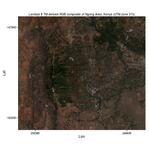
Using R’s ggplot2 library, An RGB composite can then be plotted as follows:
1
2
3
4
5
6
7
8
9
ggplot(data=mb_df, aes(x=x, y=y, fill=rgb(r,g,b, maxColorValue = 255))) +
coord_equal() + theme_bw() + geom_tile() + scale_fill_identity() +
scale_x_continuous(breaks=range(mb_df$x)*c(1.01, 0.99), labels=range(mb_df$x), expand = c(0,0)) +
scale_y_continuous(breaks=range(mb_df$y)*c(0.99, 1.01), labels=range(mb_df$y), expand = c(0,0)) +
theme(panel.grid=element_blank(), plot.title = element_text(size = 10))+
labs(list(title="Landsat 8 TM derived RGB composite of Ngong Area, Kenya (UTM zone 37s)", x="Lon", y="Lat"))
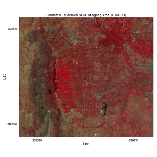
####False colour composite (FCC)
FCC’s are used to highlight particular components of the landscape e.g. certain minerals, vegetation or water bodies.
False colour compositing in R is as you might guess, just a matter of modifying how the relevant source image bands are mapped to the RGB channels of the display device.
As an example, we’ll do an RGB to NRG mapping when compositing the same image in Figure 1. This results in the so called standard false colour composite (SFCC) where vegetation features such as forests and other greenery are conspicously depicted in red, as opposed to green in true RGB compositing.
1
2
3
4
5
6
7
8
9
10
ggplot(data=mb_df, aes(x=x, y=y, fill=rgb(n,r,g, maxColorValue = 255))) +
coord_equal() + theme_bw() + geom_tile() + scale_fill_identity() +
scale_x_continuous(breaks=range(mb_df$x)*c(1.01, 0.99), labels=range(mb_df$x), expand = c(0,0)) +
scale_y_continuous(breaks=range(mb_df$y)*c(0.99, 1.01), labels=range(mb_df$y), expand = c(0,0)) +
theme(panel.grid=element_blank(), plot.title = element_text(size = 10))+
labs(list(title="Landsat 8 TM derived SFCC of Ngong Area, (UTM 37s)",
x="Lon", y="Lat"))
FCC can be extended further to highlight other landscape components. Vegetation indices and spectral ratios for minerals such as iron oxides may for example be mapped together in an RGB space to highlight the relative distribution of each component within a landscape.
References
- Liu, Jian Guo, and Philippa J. Mason. Essential image processing and GIS for remote sensing. John Wiley & Sons, 2013.
- Wickham, Hadley. ggplot2: elegant graphics for data analysis. Springer, 2016.