


####First, why bother with:
1- Reprojections?
- So that we can integrate MODIS data with other spatial data that’s in more common CRS. In this tutorial, we’ll reproject MCD43A4 HDF data to the geographic CRS based on the WGS84 datum.
2- Spatial subsetting?
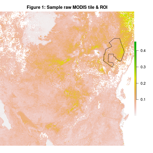
- Our region of interest (ROI) i.e. Tsavo national park is much smaller than the tile it falls in i.e. tile h21v09. We’ll thus clip our MCD43A4 HDF files to the park’s extent. Below is an outline of our ROI within a sample MCD43A4 image (band 1).
3- Spectral subsetting?
- From MCD43A4’s 7 bands, we’ll extract bands 1 (Red), 4 (Green), 3 (Blue) and 2 (NIR). This set of bands can be used for RGB & SFCC image compositing as well as in the calculation of vegetation indices.
Subsetting your data to retain only what you need:
- saves storage space
- amount of computational resources needed for subsequent processing & analysis.
###Tutorial data
The demonstration dataset was obtained from NASA’s EOSDIS through Reverb Echo.
-
Product: MODIS BRDF adjusted surface reflectance MCD43A4
-
Temporal coverage: 2001-2014. Note that MCD43A4 is produced using the “Phased production strategy”. This means that you get 46 images per year with a “running” 8 day overlap so you might want to isolate one 16 day stream from the collection, especially if you will be using the data in the form of a time series.
-
Spatial coverage: MODIS tile h21v09
The data can be explored as follows.
- Load required spatial data libraries.
1
2
3
4
5
library("raster")
library("rgeos")
library("maptools")
library("maps")
library("rgdal")
- Read sample band from a sample hdf into a raster object in R as shown below.
- Note that plotting “b01” below yields Figure 1.
1
2
bn1 <- "MOD_Grid_BRDF:Nadir_Reflectance_Band1"
b01 <- raster(readGDAL(paste("HDF4_EOS:EOS_GRID:","01_MCD_R_Shell_MRT/MCD43A4.A2005113.hdf",":", bn1, sep = ""),silent=T))
- Checking current projection
1
b01@crs
## CRS arguments:
##  +proj=sinu +lon_0=0 +x_0=0 +y_0=0 +a=6371007.181 +b=6371007.181
## +units=m +no_defs- Checking current spatial extent
1
extent(b01)
## class       : Extent
## xmin        : 3335852
## xmax        : 4447802
## ymin        : -1111951
## ymax        : 0
###Batch reprojecting MODIS HDF-EOS with R, SHELL and MODIS MRT
Requirements:
-
An R installation (obviously)
-
MODIS MRT tool installation
-
A UNIX shell e.g. BASH. Windows users can install & run BASH using CYGWIN
Next we write a function “fun_mrt” to do tasks 1-3 above. It contains 3 args:
-
“in.dir”: path to directory with input HDF files to be processed
-
“out.dir”: output directory
-
“prm.path”: path to parameter file that contains the processing parameters e.g. Here is what my parameter file, “mcd43a4.prm”, looks like:
1
2
3
4
5
6
7
8
9
10
11
12
13
14
15
16
17
18
19
20
21
22
23
INPUT_FILENAME = /home/shekeine/Projects/data/MCD43A4_h21v09/hdf/MCD43A4.A2000177.hdf
SPECTRAL_SUBSET = ( 1 1 1 1 1 1 1 )
SPATIAL_SUBSET_TYPE = INPUT_LAT_LONG
SPATIAL_SUBSET_UL_CORNER = ( -1.8 37.6 )
SPATIAL_SUBSET_LR_CORNER = ( -4.3 39.5 )
OUTPUT_FILENAME = /home/shekeine/Projects/data/MCD43A4_tsavo/sample.hdf
RESAMPLING_TYPE = NEAREST_NEIGHBOR
OUTPUT_PROJECTION_TYPE = GEO
OUTPUT_PROJECTION_PARAMETERS = (
0.0 0.0 0.0
0.0 0.0 0.0
0.0 0.0 0.0
0.0 0.0 0.0
0.0 0.0 0.0 )
DATUM = WGS84)
And behold, the function:
1
2
3
4
5
6
7
8
9
10
11
12
13
14
15
16
17
18
19
20
21
22
23
24
25
26
27
28
29
30
31
fun_mrt <- function(in.dir, prm.path, out.dir){
INLIST <- list.files(path=in.dir, full.names=T)
INNAMES<- list.files(path=in.dir, full.names=F)
for (i in 1: length(INLIST)){
#Call to sh and mrt to subset, reproject from sin to epsg 4326 and rewrite all hdf's
system(
command=paste(paste("cd ", out.dir, "&&", sep=""),
#Write hdf file to text file
paste("echo ", INLIST[i], " > ", out.dir, "/mosaicinput.txt","&&", sep=""),
#Run mrt mosaic and write output to HDF file
paste("mrtmosaic -i ", out.dir, "/mosaicinput.txt -o ", out.dir, "/mosaic_tmp.hdf","&&", sep=""),
#Call resample
paste("resample -p ", prm.path, " -i ", out.dir, "/mosaic_tmp.hdf -o ", out.dir, "/", INNAMES[i],"&&",sep=""),
paste("exit 0"), sep=""), intern=T)
print(paste("Done processing:", INNAMES[i]))
}
#Clean up working files
file.remove(paste(out.dir,"/mosaic_tmp.hdf", sep=""))
file.remove(paste(out.dir,"/mosaicinput.txt", sep=""))
file.remove(paste(out.dir,"/resample.log", sep=""))
}
Executing fun_mrt on our HDF dataset processes it as per the settings in the parameter file.
1
fun_mrt(in.dir="/home/in", prm.path="/home/mcd43a4.prm", out.dir="/home/out")
Explore result
-
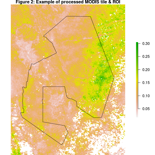
The data is now reprojected to the geographic CRS (EPSG=4326) and spatially subset to the region defined in the parameter file.
-
Spatial subsets done by “fun_mrt” can only be defined and implemented with square/rectangular ROI’s. If necessary, it is possible to clip the boundaries of the images to match those of the ROI even more closely using the
mask()function in R.
References
-
R documentation on libraries used