####Why not just stick with HDF?
1- Band math and manipulation with HDF-EOS data in R is a pain in the ear. e.g. to read a specific band (e.g. band 1 from MODIS MCD43A4) into R, one has to:
1
2
bn1 <- "MOD_Grid_BRDF:Nadir_Reflectance_Band1"
b01 <- raster(readGDAL(paste("HDF4_EOS:EOS_GRID:","02_HDF_2_mband_geotiff/hdf_in /MCD43A4.A2001033.hdf",":", bn1, sep = "")), silent=T)
- Imagine the mess you would have if you had to do a lot of band math or manipulations with hyperspectral data. Besides, the reference to band ID’s by name (rather than index position) will have you pulling your hair out if the input data changes to some other product with different band names.
2- There are dedicated tools to work with HDF-EOS data formats..
- However, if you are going to do your modelling and statistical anaylsis in R, you might as well pre-process your data within R. Who wants to keep shuttling between 10 different programs and twice as many folders between data preparation and results? Not me.
So, we agree that it would be nice to have a neat way to convert whole HDF-EOS files as multi-band raster objects in R. My solution is to write an R function that can stack all the dimensions of a batch of input HDF-EOS into multi-band GeoTIFFs for which R (and any other sensible data language or GIS) has excellent support.
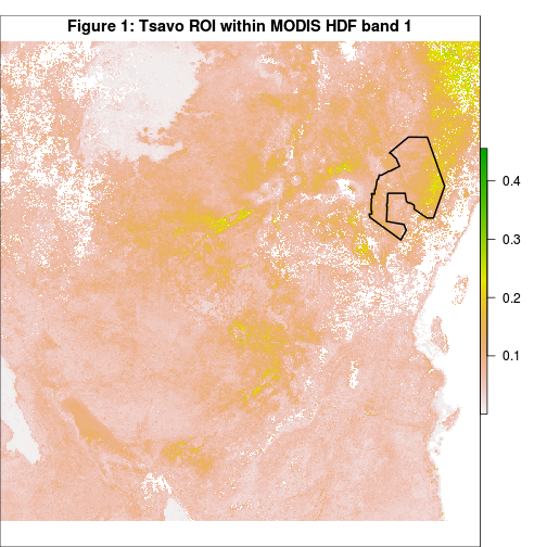
Just to get a feel of the data used in this post, we can plot the image band read in above and overlay an outline of our region of interest (ROI) as follows:
1
2
3
4
5
6
7
8
9
10
11
12
13
14
#Plot band 1 from MCD43A4.A2001033.hdf
par(mar=c(0,0,1,0))
plot(b01, axes=F)
#Import Tsavo ROI shapefile
tsavo_diss <- readShapePoly(fn="02_HDF_2_mband_geotiff/tsavo_park_diss.shp",
proj4string=CRS("+proj=longlat +datum=WGS84"))
#Transform Tsavo CRS to match b01
tsavo.sin <- spTransform(x=tsavo_diss, CRSobj=b01@crs)
#Overlay Tsavo ROI
plot(tsavo.sin, add=T, asp=1, lwd=2)
title("Figure 1: Tsavo ROI within MODIS HDF band 1", line=-1)

###Tutorial data
We’ll use the same HDF data as that in this post. Load the required libraries as shown below.
1
2
3
4
5
library("raster")
library("rgeos")
library("maptools")
library("maps")
library("rgdal")
###HDF-EOS to multi-band raster with R, SHELL and MODIS MRT
Requirements:
-
An R installation (obviously)
-
A UNIX shell e.g. BASH. Windows users can install & run BASH using CYGWIN
Next we write a function “hdf2mband” to do the work for us. It contains 4 args:
-
“in.dir”: path to directory with input HDF files to be processed
-
“out.dir”: output directory
-
“prm.path”: path to parameter file. We’ll use the same parameter file as the one here, but with line 10 ending in “.tif” instead of “.hdf”.
-
nbands: number of spectral bands in your HDF-EOS data. This argument controls how the the output bands are aggregated into multi-band rasters. That means the “nbands” value should be equal to the number of 1’s in the arg “SPECTRAL_SUBSET” of the parameter file. Otherwise expect unexpected behaviour.
And behold, the function:
1
2
3
4
5
6
7
8
9
10
11
12
13
14
15
16
17
18
19
20
21
22
23
24
25
26
27
28
29
30
31
32
33
34
35
36
37
38
39
40
41
42
43
44
45
46
47
48
49
50
51
52
53
54
55
56
57
hdf2mband <- function(in.dir, prm.path, out.dir, nbands){
INLIST <- list.files(path=in.dir, full.names=T)
INNAMES<- list.files(path=in.dir, full.names=F)
#Manufacure output names with .tif extension
OUTNAMES <- INNAMES
for (i in 1:length(OUTNAMES)){OUTNAMES[i] <- gsub(pattern=".hdf", x=OUTNAMES[i], replacement=".tif")}
for (i in 1:length(INLIST)){
#Call mrt to subset and reproject from sinusoidal to geographic CRS
system(
command=paste(paste("cd ", out.dir, "&&", sep=""),
#Write hdf file to text file
paste("echo ", INLIST[i], " > ", out.dir, "/mosaicinput.txt","&&", sep=""),
#Run mrt mosaic and write output to hdf file
paste("mrtmosaic -i ", out.dir, "/mosaicinput.txt -o ", out.dir,
"/mosaic_tmp.hdf","&&", sep=""),
#Call resample
paste("resample -p ", prm.path, " -i ", out.dir, "/mosaic_tmp.hdf -o ",
out.dir, "/", OUTNAMES[i], "&&",sep=""),
paste("exit 0"), sep=""), intern=T
)
print(paste("Done processing:", INNAMES[i]))
}
#Clean up working files
file.remove(paste(out.dir,"/mosaic_tmp.hdf", sep=""))
file.remove(paste(out.dir,"/mosaicinput.txt", sep=""))
file.remove(paste(out.dir,"/resample.log", sep=""))
#Aggregate single bands to multiband rasters
band.paths <- list.files(path=out.dir, full.names=T)
repeat{
stack.i <- stack()
for (i in 1:nbands){stack.i <- addLayer(stack.i, i=read.ras(x=band.paths[i]))}
writeRaster(x=stack.i, filename=paste(out.dir, "/",
OUTNAMES[1], sep=""), format="GTiff", overwrite=TRUE)
file.remove(band.paths[1:nbands])
#Truncate done jobs
band.paths <- band.paths[-(1:nbands)]
OUTNAMES <- OUTNAMES[-1]
if(length(band.paths)==0)
break
}
}
Executing hdf2mband processes the input HDF-EOS dataset as per the settings in the parameter file and arguments supplied to “hdf2mband”:
1
hdf2mband(in.dir=hdfin, nbands=7, prm.path=prm.path, out.dir=out.dir)
Explore result
1
2
3
4
5
#Load sample output image in R
mb_ras <- stack("02_HDF_2_mband_geotiff/mband_out/MCD43A4.A2014177.tif")
#Check number of bands, In this example, they should be 7, remember?
nlayers(mb_ras)
## [1] 71
2
3
#Define the no data fill value for the MCD43A4 product: 32767, then plot all bands
NAvalue(mb_ras) <- 32767
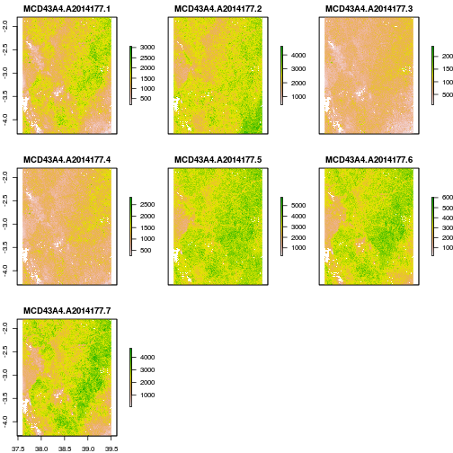
plot(mb_ras)

- Note that the final output is determined not only by the “hdf2mband” function args but also by the settings of the parameter file used e.g. “hdf2mband.prm” here. You can edit this to anything sensible to get multi-band GeoTIFFS in whatever projection, spatial or spectral extent you want.
One way to visually validate the output would be to plot an RGB composite of one of the output GeoTIFFs like the one above. How to do that will be the subject of my next post =).
References
-
R documentation on libraries used
